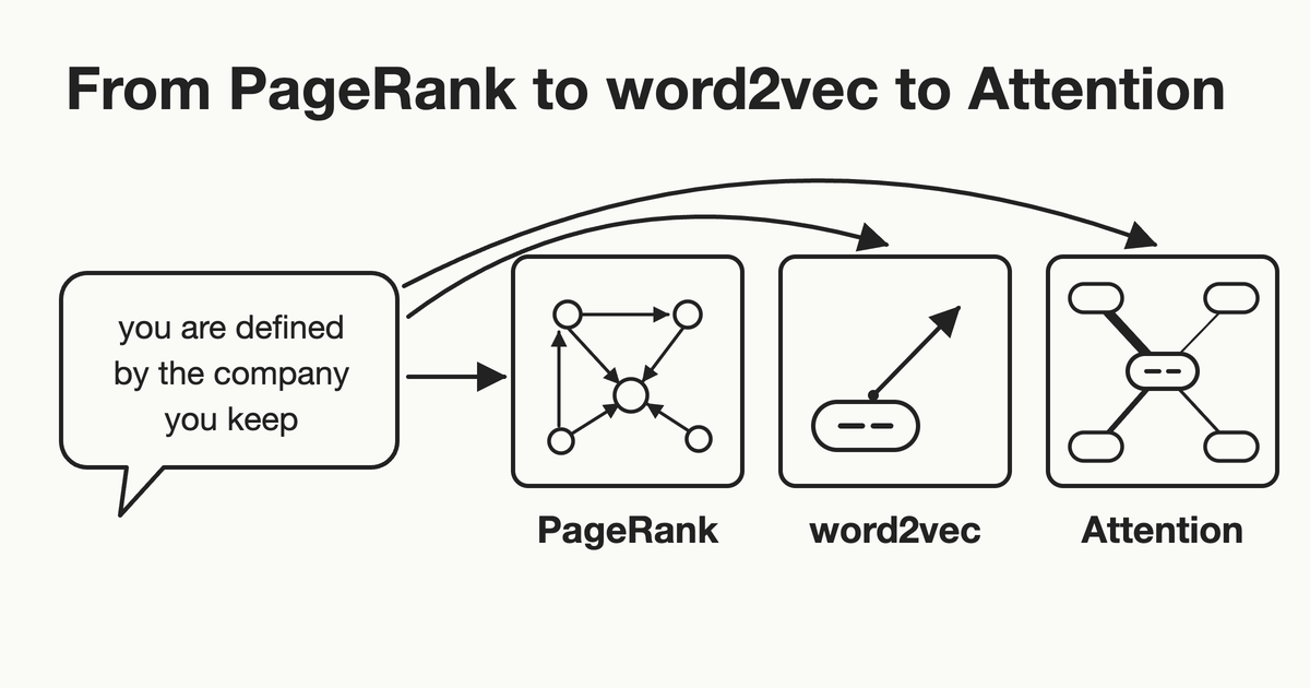
One old saying, three algorithms
Physics is easy, life is hard
At Fermi, my colleague Madhu taught a physics lesson on why physics is easy and life is hard. He talked about stable equilibrium. He said simple harmonic motion is the foundation of physics.
It sounds like an exaggeration until you see why. Pull almost anything a little away from a stable equilibrium. For small moves, the force pulling it back grows in proportion to how far it moved. That is simple harmonic motion. A pendulum, a spring, a sound wave and an atom vibrating in a crystal follow the same equation, with different knobs. The physicist Sidney Coleman is often quoted joking that the career of a young theoretical physicist is treating the harmonic oscillator in ever-increasing levels of abstraction.
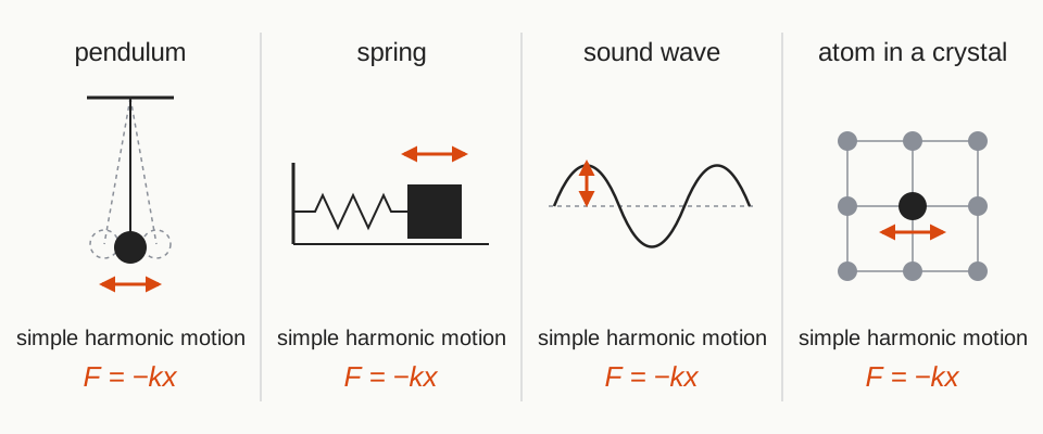
A pendulum, a spring, a sound wave and an atom in a crystal: the same equation, with different knobs.
One building block, used again and again: that is the intuition I have about my own field.
Is minimax even relevant?
I was explaining PageRank to Tanmay: in-links, out-links and the power iteration. Somewhere in that conversation he made a point. In college we learn basic things, like the minimax algorithm. He felt they are not really relevant anymore.
I disagreed. You need to understand the foundations to build your intuition. When you have that intuition, you can apply it.
So what is the simple harmonic motion of search and recommendations? I think it is one old saying, and it shows up in three famous algorithms. Each one keeps the last one and changes as little as it can.
The way I tell it is borrowed from a paper I really like, Burges’s From RankNet to LambdaRank to LambdaMART1. He never starts over. Every section keeps the previous model, changes one block, and shows you only what changed. I will do the same.
The saying
People say: you are defined by the company you keep. It is a philosophy, not an algorithm. It says what something is, in terms of its neighbours. The interesting part is what happens when you turn it into math. Two famous algorithms did exactly that, each with its own version of the saying. A third one fixed what they missed.
PageRank: the saying, for web pages
PageRank’s2 version came from how academics judge papers: a paper matters if important papers cite it. For the web:
A page is important if important pages link to it.
Read it again. The definition uses itself. To know how important a page is, you need to know how important the pages pointing to it are. That sounds circular, and it is. Math can still solve it, in three steps.
Step 1: put it in a matrix. Let’s say there are $N$ pages. Page $j$ splits its importance equally among the pages it links to. Write that as a matrix $M$, where $M_{ij} = 1/\text{outlinks}(j)$ if $j$ links to $i$, and $0$ otherwise. If $r$ is the vector of importance scores, the saying becomes one line:
$$r = M r$$
The scores are the ones that do not change when every page passes its score along its links. That is a fixed point. In linear algebra terms, $r$ is an eigenvector of $M$ with eigenvalue 1.
Step 2: fix what breaks. A group of pages that only link to each other traps all the score. The fix is the random surfer: someone who clicks links, but now and then gets bored and jumps to a random page. With probability $d$ (0.85 in the original paper) they follow a link. Otherwise they jump:
$$r = \frac{1-d}{N} + d\,M r$$
A page with no out-links is a dead end, and its score leaks away. The usual fix is to treat it as linking to every page. Our small example has no dead ends, so we can skip that here.
Step 3: solve it the simplest way. We do not need an eigen-solver. Start with equal scores, apply the formula, and repeat until the scores stop moving. This is power iteration. Here it is on a four-page web:
| |
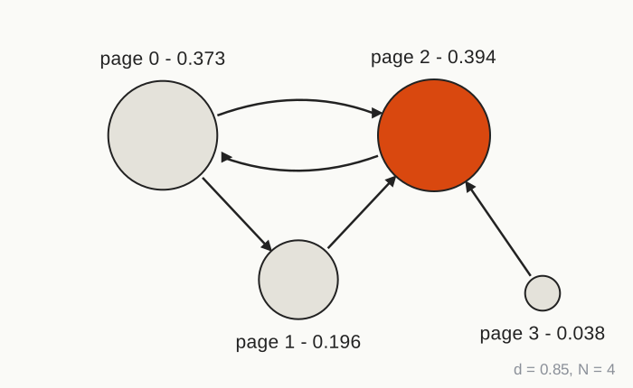
The four-page web after power iteration. Page 0 has only one in-link, but it comes from page 2, so it comes second.
Page 2 has three pages linking to it, so it wins. Page 3 has none, so it only gets the surfer’s random jumps. The interesting one is page 0. Only one page links to it, but that page is page 2, the most important one. So page 0 comes second. That is the circular definition at work.
Now look at the choices we made on the way. What counts as a link. How a page splits its score. What the surfer does when bored. How we solve it. Each of these is a knob. Keep that in mind.
word2vec: the same saying, for words
word2vec’s version of the saying is older than the computers that could use it:
You shall know a word by the company it keeps. (J. R. Firth, 19573)
Harris wrote about the distributional structure of language4 a few years before. The idea later got the name distributional hypothesis: words that appear in the same places mean similar things.
The property is different from PageRank’s. Firth is about similarity. PageRank is about importance. But the shape is the same: a thing is defined by its neighbours. So what changes when we go from pages to words?
The matrix changes. Instead of “page $j$ links to page $i$”, we count “word $c$ appears near word $w$”, inside a small window of text. That gives a co-occurrence matrix, with one row and one column for every word in the vocabulary.
What we want changes. PageRank wants one number per page: how important it is. Here we want a vector per word: what it means. Two words should get similar vectors if they keep similar company.
The solver changes. For a vocabulary of a million words, that matrix has a trillion cells. So word2vec5 never builds it. It reads text one window at a time. For each word, it pulls the word’s vector closer to the vectors of the words around it. It also pushes it away from a few random words (negative sampling6). It is stochastic gradient descent, one small step per window, over a few passes through the text.
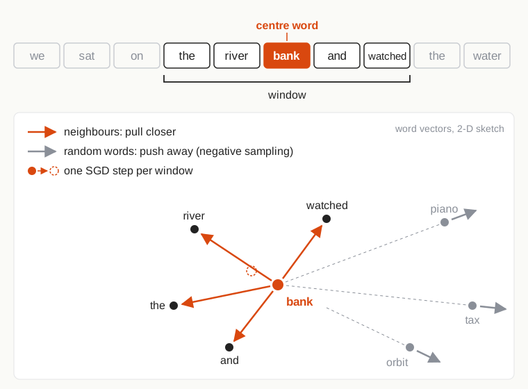
word2vec reads one window at a time. It pulls a word toward its neighbours and pushes it away from a few random words.
That looks like a completely different algorithm. It is not. Under the hood, word2vec is still working on a matrix of which words appear with which7.
So the comparison with PageRank holds, block by block:
| PageRank | word2vec | |
|---|---|---|
| The saying | a page is important if important pages link to it | words that keep similar company mean similar things |
| The matrix | links between pages | co-occurrence of words |
| What we want | one score per page | one vector per word |
| How we solve it | power iteration to a fixed point | SGD, which in effect factorizes that matrix |
Later the two ideas met. DeepWalk8 and node2vec9 take a graph and walk randomly on it, like the PageRank surfer. They write down the walks as if they were sentences, and run word2vec on them. The result is a vector for every node.
Attention: what the matrix throws away
In both algorithms, the company is flattened into one matrix. In word2vec, for a pair of words, there is one number: how often they appear together. Every word in the window is treated the same way, apart from a fixed discount for distance. And every word gets one vector, whatever sentence it is in. “Bank” in “river bank” and “bank” in “bank loan” get the same vector, because the matrix added both kinds of company into one row.
So ask the question the saying asks: which company? The neighbours do not all matter equally, and which ones matter depends on the sentence.
Let’s change that. Instead of treating every neighbour the same, take a weighted average of them. Let the weights be a learned function of the word and its neighbours. Now “bank” looks at “river” and gets one meaning, and looks at “loan” and gets another.
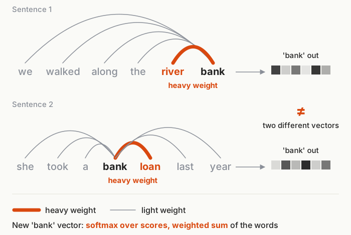
Attention chooses the company per sentence. ‘Bank’ looks at ‘river’ in one sentence and at ’loan’ in the other.
That is the core of attention. Bahdanau and co-authors first used it to let a translation model look back at the right source words10. The Transformer built the whole model out of attention over the sentence itself: self-attention11. For each word, it scores every word in the sentence, itself included. A softmax turns the scores into weights. The word’s new vector is the weighted sum of what its neighbours carry.
The meaning of a word is still defined by its company. The company is now chosen per sentence, by a function that is learned. To be honest, this step changes more than one block. The training objective and the depth of the model change too. But the block that changes the meaning of “company” is the weighting.
When I first thought this through, I got as far as: maybe word2vec, instead of a global average, could have a weighted average, or a function embedded in there. That is attention, and I missed it at the time. But that is the point: at each step you get down to a deeper nuance, and the building blocks lead you to new algorithms.
Why the building blocks matter
Let’s step back and look at what we did. We took a philosophy, turned it into math, and solved it in the simplest setup. Then we changed the blocks, step by step:
- What counts as company: links, then words in a window, then words chosen by attention.
- What we want back: a score, then a vector, then a vector per sentence.
- How we solve it: power iteration, then SGD, then a network trained end to end.
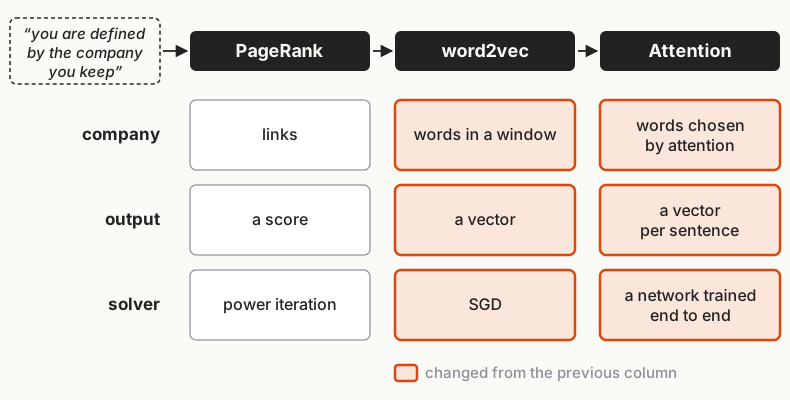
Three algorithms, one saying.
At each step there was a choice. You can only see the choices if you understand the basic setup and why it works. If you do not, you take what somebody built and apply it, or extend it a little.
This is the kind of intuition Hinton is known for. Take dropout. The paper by Srivastava, Hinton and co-authors12 starts from an idea in evolution. Sexual reproduction mixes genes, so a gene cannot rely on one exact set of partners. It has to be useful on its own. Randomly dropping units while training does the same to a network. A philosophy, then a mechanism.
Where I have used this
Two times I have used this way of thinking in my own work.
Walmart, 2014: sharing clicks between neighbouring queries. The usual way to use click engagement is one query at a time: a query, the items it returns, and the clicks on those items. I built a graph over queries instead. Each query was connected to its neighbours by a weighted, probabilistic similarity. I think it was a function of things like text overlap and queries that came up in the same sessions. Click engagement was then shared with the neighbours, along those weights. If you search for “Samsung TVs”, some of what we know about which TVs people click for “TVs” carries over.
A cousin in the literature is random walks on the click graph13, which walk between queries and the documents clicked for them. Mine linked queries to queries directly. It is the same shape as PageRank: a node’s score depends on its neighbours, spread along weighted edges.
Needl, 2024: picking context for an LLM. The usual way to fit a long document into an LLM is chunking, and chunking loses important sentences. I used a TextRank-style approach14 instead: sentences as nodes, edges from how similar they are, and the most central sentences kept as context. That is PageRank with sentences as the pages.
Both came the same way: understand the basic setup really well, then extend it.
C. J. C. Burges, From RankNet to LambdaRank to LambdaMART: An Overview, Microsoft Research Technical Report MSR-TR-2010-82, 2010. ↩︎
S. Brin and L. Page, The Anatomy of a Large-Scale Hypertextual Web Search Engine, 1998. ↩︎
J. R. Firth, A Synopsis of Linguistic Theory 1930-1955, 1957. ↩︎
Z. Harris, Distributional Structure, Word, 1954. ↩︎
T. Mikolov et al., Efficient Estimation of Word Representations in Vector Space, 2013. ↩︎
T. Mikolov et al., Distributed Representations of Words and Phrases and their Compositionality, NeurIPS 2013. ↩︎
For the curious: O. Levy and Y. Goldberg, Neural Word Embedding as Implicit Matrix Factorization (NeurIPS 2014), showed that skip-gram with negative sampling in effect factorizes the co-occurrence matrix rescaled by PMI (how much more often two words appear together than chance), shifted by the log of the number of negative samples. O. Levy, Y. Goldberg and I. Dagan, Improving Distributional Similarity with Lessons Learned from Word Embeddings (TACL 2015), then factorized positive PMI directly with SVD and, with the right settings, came close to word2vec. ↩︎
B. Perozzi, R. Al-Rfou and S. Skiena, DeepWalk: Online Learning of Social Representations, KDD 2014. ↩︎
A. Grover and J. Leskovec, node2vec: Scalable Feature Learning for Networks, KDD 2016. ↩︎
D. Bahdanau, K. Cho and Y. Bengio, Neural Machine Translation by Jointly Learning to Align and Translate, 2014. ↩︎
A. Vaswani et al., Attention Is All You Need, NeurIPS 2017. ↩︎
N. Srivastava, G. Hinton et al., Dropout: A Simple Way to Prevent Neural Networks from Overfitting, JMLR 2014. ↩︎
N. Craswell and M. Szummer, Random Walks on the Click Graph, SIGIR 2007. ↩︎
R. Mihalcea and P. Tarau, TextRank: Bringing Order into Texts, EMNLP 2004. ↩︎