Denoising Diffusion Models Part 3: Generating Characters and numbers with Diffusion Models

Notebook	Github Link	Colab
EMINST Denoising and Conditional generation	Colab EMNIST

Introduction

We have introduced most of the concepts in the previous two blogs. In this blog post, we will see how the concepts translate to code. If you want to check out the earlier posts, you can find them here, diffusion model intro 1, and diffusion model intro 2.

EMNIST dataset

Extended-MNIST dataset, as the name suggests, is an extension of the popular MNIST dataset. It contains labelled 28*28*1 images of handwritten English characters (upper and lower case) and numbers.

Loading data

We will use the Tensorflow datasets library to load the EMNIST dataset. The data will be loaded in batches of size 4*128, we will also normalize the data in the range of 0-1.

A part of this code is adapted from the vdm - simple diffusion example colab notebook.

 1
 2
 3
 4
 5
 6
 7
 8
 9
10
11
12
13
14
15
16
17
18
19
20
21
22
23
24
25
26
27
28
29
30
31
32
33
34
35
36
37
38
39
import jax
import jax.numpy as jnp
# using tensorflow libs to help load the dataset
import tensorflow_datasets as tfds
import tensorflow as tf
from clu import deterministic_data

dataset_builder = tfds.builder('emnist', data_dir=dataset_path)
dataset_builder.download_and_prepare()

train_split = tfds.split_for_jax_process('train+train', drop_remainder=True)

def preprocess_fn(example):
  image = tf.cast(example['image'], 'float32')
  image = tf.transpose(image, (1, 0, 2,))
  # normalizing values to 0-1 range
  image = image / 255.0
  return (image, example["label"] + 1)

batch_size = 4 * 128 if colab else 64
train_ds = deterministic_data.create_dataset(
    dataset_builder,
    split=train_split,
    rng=jax.random.PRNGKey(0),
    shuffle_buffer_size=100,
    batch_dims=[jax.local_device_count(), batch_size // jax.device_count()],
    num_epochs=None,
    preprocess_fn=lambda x: preprocess_fn(x),
    shuffle=True)

def create_input_iter(ds):
  def _prepare(xs):
    def _f(x):
      x = x._numpy()
      return x
    return jax.tree_util.tree_map(_f, xs)
  it = map(_prepare, ds)
  it = jax_utils.prefetch_to_device(it, 2)
  return it

Utilities for visualizing EMNIST data

Open section on utilities.

We will be using these utilities to print the images generated from the diffusion models.

A part of this code is adapted from the vdm - simple diffusion example colab notebook.

 1
 2
 3
 4
 5
 6
 7
 8
 9
10
11
12
13
14
15
16
17
18
19
20
21
22
23
24
25
26
27
28
29
30
31
32
33
34
35
36
37
38
39
40
41
42
43
44
45
46
47
48
49
50
51
52
53
54
55
56
57
58
59
60
61
62
63
64
65
66
67
68
69
70
71
72
73
74
75
76
77
78
79
80
81
82
83
84
85
86
87
88
89
import io
import math
from IPython.display import display_png
import matplotlib as mpl
import matplotlib.cm as cm

def imify(arr, vmin=None, vmax=None, cmap=None, origin=None):
  """Convert an array to an image.

  Arguments:
    arr : array-like The image data. The shape can be one of MxN (luminance),
      MxNx3 (RGB) or MxNx4 (RGBA).
    vmin : scalar, optional lower value.
    vmax : scalar, optional *vmin* and *vmax* set the color scaling for the
      image by fixing the values that map to the colormap color limits. If
      either *vmin* or *vmax* is None, that limit is determined from the *arr*
      min/max value.
    cmap : str or `~matplotlib.colors.Colormap`, optional A Colormap instance or
      registered colormap name. The colormap maps scalar data to colors. It is
      ignored for RGB(A) data.
        Defaults to :rc:`image.cmap` ('viridis').
    origin : {'upper', 'lower'}, optional Indicates whether the ``(0, 0)`` index
      of the array is in the upper
        left or lower left corner of the axes.  Defaults to :rc:`image.origin`
          ('upper').

  Returns:
    A uint8 image array.
  """
  sm = cm.ScalarMappable(cmap=cmap)
  sm.set_clim(vmin, vmax)
  if origin is None:
    origin = mpl.rcParams["image.origin"]
  if origin == "lower":
    arr = arr[::-1]
  rgba = sm.to_rgba(arr, bytes=True)
  return rgba

def rawarrview(array, **kwargs):
  """Visualize an array as if it was an image in colab notebooks.

  Arguments:
    array: an array which will be turned into an image.
    **kwargs: Additional keyword arguments passed to imify.
  """
  f = io.BytesIO()
  imarray = imify(array, **kwargs)
  plt.imsave(f, imarray, format="png")
  f.seek(0)
  dat = f.read()
  f.close()
  display_png(dat, raw=True)

def reshape_image_batch(array, cut=None, rows=None, axis=0):
  """Given an array of shape [n, x, y, ...] reshape it to create an image field.

  Arguments:
    array: The array to reshape.
    cut: Optional cut on the number of images to view. Will default to whole
      array.
    rows: Number of rows to use.  Will default to the integer less than the
      sqrt.
    axis: Axis to interpretate at the batch dimension.  By default the image
      dimensions immediately follow.

  Returns:
    reshaped_array: An array of shape [rows * x, cut / rows * y, ...]
  """
  original_shape = array.shape
  assert len(original_shape) >= 2, "array must be at least 3 Dimensional."

  if cut is None:
    cut = original_shape[axis]
  if rows is None:
    rows = int(math.sqrt(cut))

  cols = cut // rows
  cut = cols * rows

  leading = original_shape[:axis]
  x_width = original_shape[axis + 1]
  y_width = original_shape[axis + 2]
  remaining = original_shape[axis + 3:]

  array = array[:cut]
  array = array.reshape(leading + (rows, cols, x_width, y_width) + remaining)
  array = np.moveaxis(array, axis + 2, axis + 1)
  array = array.reshape(leading + (rows * x_width, cols * y_width) + remaining)
  return array

Setting up Diffusion Step

Setting up a diffusion step involves:

Defining a schedule for diffusion: $\alpha$
Defining variables that we will be using during denoising and diffusion steps.
Defining utilities to add noise to an image.

You can find more details about diffusion in the earlier post.

We are going to use the cosine schedule for diffusion in this example.

 1
 2
 3
 4
 5
 6
 7
 8
 9
10
11
def cosine_beta_schedule(timesteps, s=0.008):
    """
    cosine schedule as proposed in https://arxiv.org/abs/2102.09672
    """
    steps = timesteps + 1
    x = jnp.linspace(0, timesteps, steps)
    alphas_cumprod = jnp.cos(((x / timesteps) + s) / (1 + s) * jnp.pi * 0.5) ** 2
    alphas_cumprod = alphas_cumprod / alphas_cumprod[0]
    betas = 1 - (alphas_cumprod[1:] / alphas_cumprod[:-1])
	# clipping this at 0.1 as I have found it difficult to work with higher values of beta.
    return jnp.clip(betas, 0.0001, 0.1)

Setting up the variables:

 1
 2
 3
 4
 5
 6
 7
 8
 9
10
11
12
13
14
15
16
17
18
19
20
timesteps = 250
betas = cosine_beta_schedule(timesteps)
alphas = 1 - betas
alphas_ = jnp.cumprod(alphas, axis=0)
variance = 1 - alphas_
sd = jnp.sqrt(variance)

# these variables are used during diffusion and denoising step
alphas_prev_ = jnp.pad(alphas_[:-1], [1, 0], "constant", constant_values=1.0)
sigma_squared_q_t = (1 - alphas) * (1 - alphas_) / (1 - alphas_prev_)
log_sigma_squared_q_t = jnp.log(1-alphas) + jnp.log(1-alphas_) - jnp.log(1-alphas_prev_)
sigma_squared_q_t_corrected = jnp.exp(log_sigma_squared_q_t)

## following code here -- we are computing the posterior variance
## https://github.com/hojonathanho/diffusion/blob/1e0dceb3b3495bbe19116a5e1b3596cd0706c543/diffusion_tf/diffusion_utils_2.py#L196

## https://github.com/hojonathanho/diffusion/blob/1e0dceb3b3495bbe19116a5e1b3596cd0706c543/diffusion_tf/diffusion_utils_2.py#L78 
log_posterior_variance = jnp.log(jnp.hstack([posterior_variance[1], posterior_variance[1:]]))

posterior_variance_corrected = jnp.exp(log_posterior_variance)

Let’s define the utilities as well, adding noise using the re-parameterization trick. The diffusion step takes in data, time step value and adds noise to the data according to the equation below. It uses the schedule $\alpha$ defined above.

$$ \begin{align} q_t(x_t|x_0) &= \sqrt{\bar\alpha_t}x_0 + \sqrt{(1 - \bar\alpha_t )}\ast\epsilon_0^\ast ; \space where \space \epsilon_0^\ast \in N(0, I) \cr &= N(\sqrt{\bar\alpha_t}x_0, (1 - \bar\alpha_t)I) \cr \end{align} $$

 1
 2
 3
 4
 5
 6
 7
 8
 9
10
11
12
13
14
15
# how to add noise to the data
@jax.jit : jit compilazation to significantly speed up code
def get_noisy(rng, batch, timestep):
    timestep = einops.repeat(timestep, 'b -> b 28 28 1')
    # we will use the reparameterization trick
    # need to generate new keys everytime
    _, noise_key = jax.random.split(rng)
    noise_at_t = jax.random.normal(noise_key, shape=batch.shape)
    added_noise_at_t = jnp.add(batch * jnp.sqrt(alphas_[timestep]), noise_at_t * sd[timestep])
    return added_noise_at_t, noise_at_t

# recovering original data by removing noise
def recover_original(batch, timestep, noise):
    true_data = jnp.subtract(batch, noise*sd[timestep])/(jnp.sqrt(alphas_[timestep]))
    return true_data

Take a random data point and add noise over multiple steps. Click to see the code.

 1
 2
 3
 4
 5
 6
 7
 8
 9
10
11
12
13
14
15
16
17
18
random_index = 22
image = next(create_input_iter(train_ds))[0][0][random_index]
fig = plt.figure()
ims = []
noisy_images, _ = get_noisy(key, einops.repeat(image, 'h w c -> b h w c', b=timesteps//5), jnp.arange(1, timesteps, 5))
if colab:
  noisy_images = einops.rearrange(noisy_images, 'b h w c -> b h (w c)')
noisy_images = unnormalize(noisy_images)

for i in range(timesteps//10):
    im = plt.imshow(noisy_images[i], cmap="gray", animated=True)
    ims.append([im])

animate = animation.ArtistAnimation(fig, ims, interval=5, blit=True, repeat_delay=3000)
animate.save(gifs_dir+'diffusion.gif', writer='pillow')

with open(gifs_dir + 'diffusion.gif','rb') as f:
  display(Image(data=f.read(), format='png'))

Figure 2: Using the utilities defined above to add Gaussian Noise in multiple steps to a handwritten character ‘z’

The Denoising Model: U-Net

In the earlier blog posts, we were working on 2-d samples. The denoising model was a multi layer perceptron with GeLU activations. In the case of EMNIST we will have to denoise images. U-Nets are the recommended models to do this.

Figure 3: U-Net architecture. It’s similar to the one we will build.

The U-Net architecture has the following characteristics:

It’s typically represented as a U block.
The first part of the U block downsamples the image. We go from a 28*28 image to a 7*7 image. This is done using Downsampling convolution blocks.
With downsampling, we increase the number of channels (features). We go from 1 channel in the input to 192 channels at the end of the first part of the U-net.
The 2^nd part of the U block does the opposite of the 1st part. We go from a 7*7 image to a 28*28 image, and also go from 192 channels to 1 channel. Upsampling is done using Upsampling convolutional blocks.
At the same time, the U-Net has residual connections, connecting layers in the downsampling part to the layers in the upsampling part, this makes training the network efficient.

 1
 2
 3
 4
 5
 6
 7
 8
 9
10
11
12
13
14
15
16
17
18
19
# upsample operation in the UNET
class Downsample(hk.Module):
  def __init__(self, output_channels):
    super().__init__()
    self.conv = hk.Conv2D(output_channels=output_channels, kernel_shape=(4, 4), stride=2, padding=[1, 1])
  
  def __call__(self, x):
    return self.conv(x)
  
# Downsample operation in the UNET
class Upsample(hk.Module):
  def __init__(self, output_channels):
    super().__init__()
    self.conv = hk.Conv2D(output_channels=output_channels, kernel_shape=(3, 3), padding='SAME')
  
  def __call__(self, x):
    # scaling image to twice size
    x = einops.repeat(x, 'b h w c -> b (a h) (aa w) c', a=2, aa=2)
    return self.conv(x)

Time Step Embeddings: We will be using sinusoidal embeddings for time steps. This is following the discussion in the previous post.

 1
 2
 3
 4
 5
 6
 7
 8
 9
10
11
12
class TimeEmbeddings(hk.Module):
  def __init__(self, dim):
    super().__init__()
    half_dim = dim // 2
    embeddings = math.log(10000) / (half_dim - 1)
    self.embeddings = jnp.exp(jnp.arange(half_dim) * -embeddings)

  def __call__(self, timesteps):
      embeddings = self.embeddings
      embeddings = jnp.multiply(timesteps[:, None], embeddings[:, None].T)
      embeddings = jnp.hstack([jnp.sin(embeddings), jnp.cos(embeddings)])
      return embeddings

Conditional Labels: EMNIST dataset has 62 labels, 26 characters in lowercase, 26 characters in uppercase, 10 numbers. We add another label to represent the masked label. We use the Haiku Embed class to generate embedding vectors for these labels. Labels are fused with the input as explained in the previous post. Instead of fusing label and time step information only at the start, we are fusing it with the input at every Block.

Network Definition: After convolution layers, I am using a BatchNorm¹ layer, using the Haiku BatchNorm module to normalize the values across the batch. This is shown to improve the convergence of deep models. Using BatchNorm complicates the implementation a bit since, BatchNorm layers need to maintain a buffer states for mean and variance of the activations. This video from Yannic is an excellent introduction to the different kind of Normalizations that one can apply to speed up training.

The code below follows the U-net implementation in LucidRains Diffusion model implementation.

 1
 2
 3
 4
 5
 6
 7
 8
 9
10
11
12
13
14
15
16
17
18
19
20
21
22
23
24
25
26
27
28
29
30
31
32
33
34
35
36
37
38
39
40
41
42
43
44
45
46
47
48
49
50
51
52
53
54
55
56
57
58
59
60
61
62
63
64
65
66
67
68
69
70
71
72
73
74
75
76
77
78
79
80
81
82
83
# Unet class to predict noise from a given image
class UNet(hk.Module):
  def __init__(self):
    super().__init__()
    self.init_conv = hk.Conv2D(output_channels=48, kernel_shape = (5,5), padding='SAME', with_bias=False)
    self.norm = hk.BatchNorm(True, True, decay_rate=0.9)
    self.silu = jax.nn.silu
    self.block1 = Block(output_channels=48, kernel_size=3, padding=1)
    self.downsample1 = Downsample(96)
    self.block2 = Block(output_channels=96, kernel_size=3, padding=1)
    self.downsample2 = Downsample(192)
    self.middle_block = Block(output_channels=192, kernel_size=3, padding=1)
    self.upsample1 = Upsample(96)
    self.block3 = Block(output_channels=96, kernel_size=3, padding=1)
    self.upsample2 = Upsample(48)
    self.block4 = Block(output_channels=48, kernel_size=3, padding=1)
    self.conv1 = hk.Conv2D(output_channels=48, kernel_shape = (3,3), padding='SAME', with_bias=False)
    self.norm1 = hk.BatchNorm(True, True, decay_rate=0.9)
    self.conv2 = hk.Conv2D(output_channels=1, kernel_shape = (5,5), padding='SAME')
    
    self.time_mlp = hk.Sequential([
      hk.Linear(256),
      jax.nn.gelu,
      hk.Linear(256),
    ])
    # conditional vectors encoding
    self.embedding_vectors = hk.Embed(10+26+26+1, 63)
    self.timestep_embeddings = TimeEmbeddings(96)
      
  def __call__(self, x, timesteps, cond=None, is_training=False):
    cond_embedding = None
    conditioning = None
    if timesteps is not None:
      timestep_embeddings = self.timestep_embeddings(timesteps)
      conditioning = timestep_embeddings
    if cond is not None:
      label_embeddings = self.embedding_vectors(cond)
      conditioning = jnp.concatenate([label_embeddings, conditioning], axis=1)
    if conditioning is not None:  
      cond_embedding = self.time_mlp(conditioning)
    h = self.silu(self.norm(self.init_conv(x), is_training))
    xx = jnp.copy(h)
    b1 = self.block1(h, cond_embedding, is_training)
    h = self.downsample1(b1)
    b2 = self.block2(h, cond_embedding, is_training)
    h = self.downsample2(b2)
    h = self.upsample1(self.middle_block(h, cond_embedding, is_training))
    b3 = self.block3(jnp.concatenate((h, b2), axis=3), cond_embedding, is_training)
    h = self.upsample2(b3)
    b4 = self.block4(jnp.concatenate((h, b1), axis=3), cond_embedding, is_training)
    h = self.conv2(self.silu(self.norm1(self.conv1(jnp.concatenate((xx, b4), axis=3)), is_training)))
    return h

class Block(hk.Module):
  # a basic resnet style convolutional block
  def __init__(self, output_channels, kernel_size, padding):
    super().__init__()
    self.proj = hk.Conv2D(output_channels=output_channels, kernel_shape=(kernel_size, kernel_size), padding='SAME', with_bias=False)
    # using batch norm instead of layernorm as the batch sizes are large
    # orig: self.norm = hk.LayerNorm(axis=(-3, -2, -1), create_scale=True, create_offset=True)
    self.norm = hk.BatchNorm(True, True, decay_rate=0.9)
    self.silu = jax.nn.silu
    self.conv1 = hk.Conv2D(output_channels=output_channels, kernel_shape=(kernel_size, kernel_size), padding='SAME', with_bias=False)
    self.norm1 = hk.BatchNorm(True, True, decay_rate=0.9)
    self.out_conv = hk.Conv2D(output_channels=output_channels, kernel_shape=(1, 1), padding='SAME') 
    # self.time_mlp = None
    dims = output_channels
    self.time_mlp = hk.Sequential([
      jax.nn.silu,
      hk.Linear(dims*2),
    ])
    
  def __call__(self, x, timestep_embeddings=None, is_training=False):
    h = self.proj(x)
    h = self.norm(h, is_training)
    if timestep_embeddings is not None and self.time_mlp is not None:
      time_embedding = self.time_mlp(timestep_embeddings)
      time_embedding = einops.rearrange(time_embedding, 'b c -> b 1 1 c')
      shift, scale = jnp.split(time_embedding, indices_or_sections=2, axis=-1)
      h = shift + (scale+1)*h
    
    h = self.silu(self.norm1(self.conv1(self.silu(h)), is_training))
    return self.out_conv(x) + h

Training Code:

Loss function: I am using the Huber loss instead of using the L2 or the L1 loss. I would assume changing the loss function wouldn’t impact the results significantly.

Note: the importance weight determines the importance of the sample for denoising. As noted in Improved Denoising Diffusion Probabilistic Models², one idea to train diffusion models is to completely ignore this term. This helps the model training.

 1
 2
 3
 4
 5
 6
 7
 8
 9
10
11
12
13
14
15
16
17
18
19
20
21
22
23
# using jax.jit to speed up computation of the loss function
partial(jax.jit,  static_argnums=(4,))
def compute_loss(params: hk.Params, state: hk.State, batch: Batch, is_energy_method: bool=False, is_training=False) -> Tuple[jnp.ndarray, Tuple[jnp.ndarray, hk.State]]:
  """Compute the loss of the network, including L2."""
  x, label, timestep, noise = batch
  # not capturing state as it is not needed; it should be internally updated and maintaing by haiku and doesn't need gradient updates 
  pred_data, state = net.apply(params, state, x, timestep, label, is_training)
  
  def error_func():
    imp_weight = 1.0 # 1/2 * (1/sigma_squared_q_t_corrected[timestep]) * ((betas[timestep])**2 / (variance[timestep] * alphas[timestep]))
      # loss on prediction
    loss_ = jnp.mean(jnp.multiply(imp_weight, huber_loss(noise, pred_data)))
    return loss_
  
  def energy_func():
    ## Energy function interpretation
    imp_weight = 1.0 # 1/2 * (1/sigma_squared_q_t_corrected[timestep]) * ((betas[timestep])**2 / (alphas[timestep]))
    # loss on prediction
    loss_ = jnp.mean(jnp.multiply(imp_weight, huber_loss(pred_data, jnp.divide(noise, -sd[timestep]))))
    return loss_
    
  loss_ = jax.lax.cond(is_energy_method, energy_func, error_func)
  return loss_, (loss_, state)

Updating Model Weights:

This is a typical code for any Neural Network training in Haiku/Optax and JAX. We are finding the gradient of the loss with respect to the parameters of the Neural Network using JAX and updating the weights using Optax.

Additionally, we are doing exponential updates to the parameters. Paper on Polyak averaging.³

 1
 2
 3
 4
 5
 6
 7
 8
 9
10
11
12
13
14
15
16
17
18
@jax.jit
def update(
    params: hk.Params,
    state: hk.State,
    opt_state: optax.OptState,
    batch: Batch,
    is_energy_method: bool=False) -> Tuple[jnp.ndarray, hk.Params, optax.OptState, hk.State]:
  """Compute gradients and update the weights"""
  grads, (loss_value, state)= jax.grad(compute_loss, has_aux=True)(params, state, batch, is_energy_method, is_training=True)
  updates, opt_state = opt.update(grads, opt_state)
  new_params = optax.apply_updates(params, updates)
  return loss_value, new_params, opt_state, state

@jax.jit
def ema_update(params, avg_params):
  """Incrementally update parameters via polyak averaging."""
  # Polyak averaging tracks an (exponential moving) average of the past parameters of a model, for use at test/evaluation time.
  return optax.incremental_update(params, avg_params, step_size=0.95)

Training Code

The training code is pretty straight-forward. Below, I have removed the code to checkpoint the different models.

Pseudocode we are going for:

 1
 2
 3
 4
 5
 6
 7
 8
 9
10
11
12
13
14
15
16
17
18
19
20
21
22
def diffusion(x_0, t):
	code to add noise to x_0
	return x_i

def training():
	for loop until convergence:
		pick an image x_0 from X (batch of images)
		sample t from 1 to T
		x_t = diffusion_step(x_0, t)
		x_hat_t = NN(x_t, t, y)  # y is the label
		loss_ = loss(x_0, x_hat_t)
		update(NN, grad(loss_)

# generating new data points through denoising steps
def generate_new_data():
	sample x_T from N(0, I)
	for t in range(T, 1):
		# denoising step
		x_hat_t = NN(x_t, t, y)  # y is the desired label 
		# get x_{t-1}
		x_{t-1} = func(x_hat_t, t) # refer EQ - 12
	x_hat_0 = x_0  

 1
 2
 3
 4
 5
 6
 7
 8
 9
10
11
12
13
14
15
16
17
18
19
20
21
22
23
24
25
26
27
28
29
30
31
32
33
34
35
36
37
38
39
40
41
42
43
44
45
46
47
48
49
50
# initialization
def f(x, timesteps, label, is_training):
  unet = UNet()
  return unet(x, timesteps, label, is_training)

f_t = hk.transform_with_state(f)
net = hk.without_apply_rng(f_t)
params, state = net.init(rng, image[0][0:batch_size], timesteps_, label[0][0:batch_size], is_training=True)
opt = optax.adam(1e-3)
avg_params = deepcopy(params)
opt_state = opt.init(params)
batches_iter = 10000

# maintaining a batch on which we will measure loss; we will save the model based on performance on this batch
one_timestep = jnp.mod(jnp.arange(1, batch_size+1), timesteps)
train = create_input_iter(train_ds) 
data_in_batch_, label_ = next(train)
data_in_batch_ = data_in_batch_[0]
label_ = label_[0]
data_noisy_temp_, noise_temp_ = get_noisy(key, data_in_batch_, one_timestep)

# main method for training
def train_model(opt_state, params, avg_params, state, energy_method=False):
    best_loss = sys.float_info.max # initialization   
	unique_key = jax.random.fold_in(key, batch_size)
	
	# same subkey being used for noise sampling, as it doesn't matter :)
	_, *timestep_subkeys = jax.random.split(unique_key, batches_iter+1)
	
	losses = []
	for iteration in range(0, batches_iter):
		data_in_batch, label = next(train)
		data_in_batch = data_in_batch[0]
		label = label[0]
		idx = (jax.random.uniform(key=timestep_subkeys[iteration], shape=(batch_size, 1)) * (timesteps-1)).astype(int)
		idx = einops.rearrange(idx, 'a b -> (a b)')
		timestep = idx + 1
		data_noisy, noise = get_noisy(timestep_subkeys[iteration], data_in_batch, timestep)
		# todo: call gradient update function here
		loss_value, params, opt_state, state = update(params, state, opt_state, [data_noisy, label, timestep, noise], energy_method)
		avg_params = ema_update(params, avg_params)
		                
		## evaluating noise on a fixed timestep to calculate best model
		loss_temp, _ = jax.device_get(compute_loss(avg_params, state, [data_noisy_temp_, label_, one_timestep, noise_temp_], energy_method, is_training=False))
		losses.append(loss_temp)
	
		if loss_temp < best_loss:
			best_loss = loss_temp
			print(f"saving iteration: {iteration} loss: {best_loss:>7f}")
return data_noisy, data_in_batch, timestep, losses, avg_params, state

Generating Conditional Samples

Using all time steps for generation

Code for generating samples is below. We start off with random samples from a Standard Gaussian Distribution and follow steps as described here. We will be using the naïve version of classifier guidance described here.

Start by sampling a random image from a Sandard Gaussian distribution at time step $T$.
Get an estimate of the error added to the input image from the U-net.
Use the equation 5, in the link above, to calculate the image at the previous time step $T-1$.
Repeat until time step 1.

1
2
3
4
5
6
7
8
9
# defining useful variables
alphas_prev_ = jnp.pad(alphas_[:-1], [1, 0], "constant", constant_values=1.0)
sigma_squared_q_t = (1 - alphas) * (1 - alphas_) / (1 - alphas_prev_)
log_sigma_squared_q_t = jnp.log(1-alphas) + jnp.log(1-alphas_) - jnp.log(1-alphas_prev_)
sigma_squared_q_t_corrected = jnp.exp(log_sigma_squared_q_t)
key = jax.random.PRNGKey(42)

mean_coeff_1 = jnp.sqrt(alphas)*(1 - alphas_prev_) / variance
mean_coeff_2 = jnp.sqrt(alphas_prev_) * betas / variance

Generate Samples:

 1
 2
 3
 4
 5
 6
 7
 8
 9
10
11
12
13
14
15
16
17
18
19
20
21
22
23
24
25
26
27
28
29
30
31
32
33
34
35
import random

def generate_data(avg_params, state, label, energy_method=False, clipped_version=False):
    batch_size_generation = len(label)
    unique_key = jax.random.fold_in(key, random.randint(1, 100))
    _, subkey = jax.random.split(unique_key)
    _, *subkeys = jax.random.split(unique_key, timesteps+1)
    
    # need to generate new keys everytime
    data_noisy = jax.random.normal(subkey, shape=(batch_size_generation, 28, 28, 1))
      
    data_in_batch = data_noisy
    datas = []
    datas.append(jax.device_get(data_noisy))
    for t in range(1, timesteps+1):
        timestep = timesteps-t
        t_repeated = jnp.repeat(jnp.array([timestep]), batch_size_generation)
        # data_stacked = torch.vstack([data_in_batch, labelled_values])
        pred_data, _ = net.apply(avg_params, state, data_in_batch, t_repeated, label, is_training=False)
		# clipping an improvement as recommended in https://github.com/hojonathanho/diffusion/blob/1e0dceb3b3495bbe19116a5e1b3596cd0706c543/diffusion_tf/diffusion_utils.py#L171
		# this helps in improving the samples generated as it keeps the random variables in the range of 0 to +1
		x_reconstructed = jnp.subtract(data_in_batch, pred_data * sd[timestep])/ jnp.sqrt(alphas_[timestep])

		if timestep >= 0:
			x_reconstructed = jnp.clip(x_reconstructed, 0., 1.)

		mean_data_1 = data_in_batch * mean_coeff_1[timestep]
		mean_data_2 = x_reconstructed * mean_coeff_2[timestep]
		mean_data = jnp.add(mean_data_1, mean_data_2)

        posterior_data = posterior_variance_corrected[timestep]
        data_noisy = jax.random.normal(subkeys[t-1], shape=(batch_size_generation, 28, 28, 1))
        data_in_batch = jnp.add(mean_data,  jnp.sqrt(posterior_data) * data_noisy)
        datas.append(jax.device_get(data_in_batch))
    return datas, data_in_batch

Striding: Reducing steps needed for Generation

We could reduce the number of steps needed for generation. One of the popular approaches to do this is by using Time Step Striding.

Instead of moving stepsone at a time from $T$ to 1, range(T, 1, -1), we will move $s$ steps at a time, range(T, 1, -s). Doing this will speed up generation of new samples from the model by s times. I have been able to produce good quality samples with $s$ set to 5.

We just need to make minor adjustments to the variables we created so that the maths still works.

 1
 2
 3
 4
 5
 6
 7
 8
 9
10
11
12
strided_schedule = jnp.array(list(range(1, timesteps, 5)) + [timesteps])

alphas_strided_ = alphas_[strided_schedule]
alphas_prev_strided_ = jnp.pad(alphas_strided_[:-1], [1, 0], "constant", constant_values=1.0)

betas_strided = 1 - (alphas_strided_/alphas_prev_strided_)
posterior_variance_new_schedule = betas_strided * (1 - alphas_prev_strided_)/ (1-alphas_strided_)
log_posterior_variance = jnp.log(jnp.hstack([posterior_variance_new_schedule[1], posterior_variance_new_schedule[1:]]))
posterior_variance_new_schedule_corrected = jnp.exp(log_posterior_variance)

mean_coeff_1_strided = jnp.sqrt(1-betas_strided)*(1 - alphas_prev_strided_) / (1 - alphas_strided_)
mean_coeff_2_strided = jnp.sqrt(alphas_prev_strided_) * betas_strided / (1 - alphas_strided_)

Generate Samples:

The code to generate samples is pretty similar, now we need to use the strided variables defined above.

 1
 2
 3
 4
 5
 6
 7
 8
 9
10
11
12
13
14
15
16
17
18
19
20
21
22
23
24
25
26
27
28
29
30
31
32
33
34
import random

def generate_data_strided(avg_params, state, label, energy_method=False, clipped_version=False):
    batch_size_generation = len(label)
    unique_key = jax.random.fold_in(key, random.randint(1, 100))
    _, subkey = jax.random.split(unique_key)
    _, *subkeys = jax.random.split(unique_key, len(strided_schedule)+1)
    
    data_noisy = jax.random.normal(subkey, shape=(batch_size_generation, 28, 28, 1))
          
    data_in_batch = data_noisy
	datas = []
    datas.append(jax.device_get(data_noisy))                   
    for t in range(1, len(strided_schedule)+1):
        stride_timestep = len(strided_schedule)-t
        timestep = strided_schedule[stride_timestep]
        t_repeated = jnp.repeat(jnp.array([timestep]), batch_size_generation)
        # data_stacked = torch.vstack([data_in_batch, labelled_values])
        pred_data, _ = net.apply(avg_params, state, data_in_batch, t_repeated, label, is_training=False)
		# Clipping helps in improving the samples generated as it keeps the random variables in the range of 0 to +1
		x_reconstructed = jnp.subtract(data_in_batch, pred_data * sd[timestep])/ jnp.sqrt(alphas_[timestep])
		
		if timestep >= 0:
			x_reconstructed = jnp.clip(x_reconstructed, 0., 1.)

		mean_data_1 = data_in_batch * mean_coeff_1_strided[stride_timestep]
		mean_data_2 = x_reconstructed * mean_coeff_2_strided[stride_timestep]
		mean_data = jnp.add(mean_data_1, mean_data_2)

        posterior_data = posterior_variance_new_schedule_corrected[stride_timestep]
        data_noisy = jax.random.normal(subkeys[t-1], shape=(batch_size_generation, 28, 28, 1))
        data_in_batch = jnp.add(mean_data,  jnp.sqrt(posterior_data) * data_noisy)
        datas.append(jax.device_get(data_in_batch))
    return datas, data_in_batch

Generating Samples & Outputs

Let’s first create a map between the label values and the characters.

 1
 2
 3
 4
 5
 6
 7
 8
 9
10
11
import string

x = list(range(1, 63))
y = [str(i) for i in (list(range(0, 10)))] + list(string.ascii_uppercase + string.ascii_lowercase)

dict_ = {}
for i in x:
  dict_[y[i-1]] = i
  
def get_label(ans):
  return jnp.array([dict_[str.upper(char)] for char in ans])

Generating Samples:

Generating ‘varun’ using the trained diffusion model.

1
2
3
4
5
6
datas, d = generate_data_strided(avg_params, state, label= "varun", energy_method=False, clipped_version=True)
datas_ = jnp.clip(jnp.array(datas[0: -1 :2]), 0., 1.)
d_ = einops.rearrange(datas_, 'a b c d e -> (b a) c d e') 

rawarrview(reshape_image_batch(datas[-1].squeeze(), rows=1), cmap='bone_r')
rawarrview(reshape_image_batch(d_.squeeze(), rows=5), cmap='bone_r')

Figure 4: ‘varun’ generated using strided sampling technique.

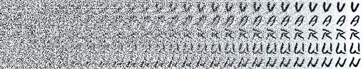
Figure 5: Visualizing the steps in the diffusion process. If you notice carefully, not much is happening at the early stages.

Generating ‘tulsian’ using the trained diffusion model.

1
2
3
4
5
datas, d = generate_data_strided(avg_params, state, label= "tulsian", energy_method=False, clipped_version=True)
datas_ = jnp.clip(jnp.array(datas[0: -1 :2]), 0., 1.)
d_ = einops.rearrange(datas_, 'a b c d e -> (b a) c d e') 
rawarrview(reshape_image_batch(datas[-1].squeeze(), rows=1), cmap='bone_r')
rawarrview(reshape_image_batch(d_.squeeze(), rows=7), cmap='bone_r')

Figure 6: ’tulsian’ generated using strided sampling technique.

Figure 7: Visualizing the steps in the diffusion process. Similar to earlier, not much is happening at the early stages.

Conclusion

Denoising Diffusion models are a powerful algorithmic tool for Generative AI. Although much of the work done so far focusses on images, we could generate any distribution using these techniques.

I sincerely hope this introduction was useful to you. Please explore additional resources here.

Want to connect? Reach out @varuntul22.

Ioffe et al. 2015 Batch Normalization: Accelerating Deep Network Training by Reducing Internal Covariate Shift ↩︎
Nichol et al. 2021 Improved Denoising Diffusion Probabilistic Models ↩︎
Polyak et al. 1991Acceleration of Stochastic Approximation by Averaging ↩︎

Introduction#

EMNIST dataset#

Loading data#

Utilities for visualizing EMNIST data#

Setting up Diffusion Step#

The Denoising Model: U-Net#

Training Code:#

Training Code#

Generating Conditional Samples#

Using all time steps for generation#

Striding: Reducing steps needed for Generation#

Generating Samples & Outputs#

Conclusion#