Code for this blog post:
| Notebook | Github Link | Colab |
|---|---|---|
| Predicting Error and Score Function | Error / Score Prediction | |
| Classifier free Guidance and other improvements | Advanced concepts |
Topics to cover
We have done most of the heavy-lifting in Part 1 of this series on Diffusion Models. To be able to use them well in practice, we may need to make some more improvements. That’s what we will do.
- Time step embedding and concatenation/fusion to the input data.
- Error Prediction $\hat \epsilon_0^\ast$ and Score Function Prediction $s$ instead of predicting the actual input $x_0$.
- Class conditioned generation or Classifier free guidance, where we guide the diffusion model to generate data based on class labels.
The ideas are an extension to the concepts introduced earlier, but are vital parts of any practical diffusion model implementation.
Time Step Embedding
During the denoising process, the Neural Network needs to know the time step at which denoising is being done. Passing the time step $t$ as a scalar value is not ideal. Rather, it would be preferable to pass the time step as an embedding to the Neural Network. In the Attention is all you need1 paper, the authors proposed sinusoidal embeddings to encode position of the tokens (time steps in our case).
Pseudocode:
| |
Sinusoidal embeddings are small in absolute value and can be fused(added) or concatenated to the input data to provide the Neural Network some information about the time step at which the denoising process is happening.
Passing Time Step Embedding (Fusing and Concatenation):
| |
Fusing the data with the data is computationally efficient as it requires significantly fewer number of weight parameters. The key idea here is that Neural Networks are powerful enough to separate any added information to the original data without the information being explicitly passed. Have a look at this video if you want to get better intuition. Positional embeddings in transformers EXPLAINED.
If we want to add time step information to an image, it is typically done by broadcasting the time step embedding along the channel dimension.
Adding Time Step to Image (Fusing):
| |
Fusing data to an input is a technique useful to add any kind of conditional information to the data. We will use this idea in EMNIST: Blog 3 where we use this concept to fuse label and time step information with the images during class conditional generation. This technique was used in the work, Improved Denoising Diffusion Probabilistic Models.
Error Prediction and Score Function Prediction
Predicting the Error $\hat \epsilon_0^\ast$
During the denoising step, the model ingests $\hat x_t$ and spits out $\hat x_t^0$, a prediction for $x_0$. Instead of outputting predictions of the input data, we want the model to output a prediction of the error $\hat\epsilon^\ast_0$.
Let’s investigate the relationship between error $\epsilon_0^\ast$ and input data $x_0$. $$ \begin{align} x_t &= \sqrt{\bar\alpha_t}x_0 + \sqrt{(1 - \bar\alpha_t )}\ast\epsilon_0^\ast \cr x_0 &= \frac{x_t-\sqrt{(1 - \bar\alpha_t )}\ast\epsilon_0^\ast}{\sqrt{\bar\alpha_t}} \end{align} $$ Equation 2 shows that if we have $x_t$ and $\epsilon^\ast_0$ than it determines $x_0$.
The denoising step now looks like this:
- Make a prediction of source error $\hat\epsilon^\ast_0$ using the $NN(\hat x_t, t)$.
- Using Equation 2, evaluate $x_0^t$, which is the prediction of the input data at time step $t$.
- Next step:
- During training: We want an equivalent version of the loss function $Error\_Loss(\epsilon^\ast_0, \hat \epsilon_0^\ast, t)$. $$ \begin{align} Loss(x_0, \hat x_t, t) = 1/2\ast(\frac{\bar\alpha_{t-1}}{1-\bar\alpha_{t-1}} - \frac{\bar\alpha_t}{1-\bar\alpha_t})\ast\mid\mid x_0-\hat x_0^t\mid\mid_2^2 \cr \text{Making modifications to loss using Equation 2} \nonumber \cr Error\_Loss(\epsilon^\ast_0, \hat \epsilon_0^\ast, t) = \frac{1}{2\sigma^2_q(t)} \frac{(1-\alpha_t)^2}{(1-\bar\alpha_t)\alpha_t}\mid\mid \epsilon^\ast_0-\hat \epsilon^\ast_0\mid\mid_2^2 \end{align} $$
- During data generation:
- Using Equation 2, reconstruct $\hat x_0^t$. Remember, $x_0$ is a function of the Gaussian error and the latent variable.
- Clip the $\hat x_0^t$ to make sure it lies in the range of -1 to +1 (normalized range for input data).
torch.clip(x_reconstructed, -1, 1) - Using Equation 5 (below) get a prediction for the latent at $t-1$ time step.
Predicting error is empirically shown to work well, refer Denoising paper2. This is probably due to the clipping of the predicted output at every time step so that the predicted data is in the normalized range. Refer this discussion.
Here is an interesting discussion on why predicting error works for images, but may not work well for other domains such as voice generation.
Another important reason is that the standard formulation everyone has ended up using for images (predict the standardised noise given noisy input) implicitly downweights high frequency components, which is an excellent match for the human visual system.
— Sander Dieleman (@sedielem) August 11, 2022
Denoising Step during data generation:
| |
Score Function Prediction
This is yet another variation on diffusion models. Similar to predicting the error as discussed earlier, we could also predict the score function. The score function $s$ is defined as $\nabla p(x_t)$.
All we need is to define $x_t$ as $f(s)$. We could then define a $Score\_Loss(s, \hat s, t)$ by substituting $x_t$ for the function $f(s)$ in the training step. In the denoising step we will use the function $f(s)$ defined to compute $x_t$, perform clipping so that the output lies in the normalized range and proceed as we did in the earlier section.
The relation between $s$ and $x$ is defined as below: $$ x_0 = \frac{x_t + (1 - \bar\alpha_t )\ast\nabla p(x_t)}{\sqrt{\bar\alpha_t}} $$
For more details and intuition on why this is an important interpretation, please refer to the section on Three equivalent interpretations.3 Yang Song has an excellent blog post on Score based generative models.
Guidance & Classifier-free Guidance
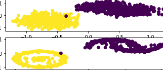
We want to control the data we generate. For example, in the image below, we have 2 labels. During generation, we want to direct the model to generate samples either from Yellow or Purple classes. Classifier Guidance is a way to do this. We will be guiding the denoising process to generate samples that are more likely to belong to the conditioned class.
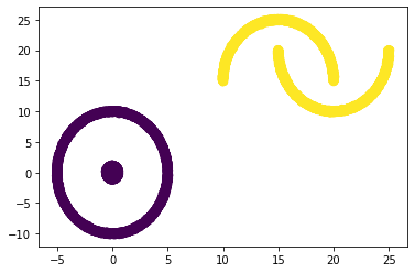
Figure 1: Data with 2 labels, Circles in Purple and Moons in Yellow
Text-guided diffusion models like Glide use the powerful Neural Network called CLIP and classifier guidance techniques to perform text-based image generation.
So far, we have been trying to maximize the likelihood of the data distribution $p(x)$ with diffusion models. This allowed us to randomly sample data points from the data distribution.
A naïve idea to do class-conditioned generation could be to fuse the conditional label information with the input data.
Pseudocode for naïve idea:
| |
During training and data generation, we will add the conditioned label as an input along with the noisy data and the time step embedding. The output of the model will stay the same as earlier.
The conditioned data can be fused with the input data, just like we fused the time step information.
| |
Guidance
The above approach may lead to models that have low sample diversity. Researchers have proposed two other forms of guidance: classifier guidance and classifier-free guidance4.
Classifier Guidance guides the generation of new samples with the help of a classifier. The classifier takes a noisy image ($x_t$) as input and predicts the label $y$. The gradient of the distribution $p(y|x)$ is used to make updates to the weights of the Neural Network to guide it to produce samples that are likely to be $y$. This is an adversarial loss, and this approach has similarities to GANs.
Classifier-Free Guidance would be ideal if we did not want to build a classifier. The classifier-free guidance approach models the conditional likelihood of samples as follows: $$ \nabla p(x|y) = \lambda \ast \underbrace{\nabla p(x|y)}_{\text{conditional}} + (1-\lambda) \ast \underbrace{\nabla p(x)}_{\text{unconditional}} $$ The conditional and the unconditional distributions are modelled by the same neural network. To model the conditional distribution, we fuse the label information as shown in the naïve approach above. To model the unconditional distribution, we mask the label information and pass it to the diffusion model. The lambda parameter, controls the diversity of the sample we want to generate. $\lambda=1$ would be equivalent to the naïve approach.
Adding this perspective about efficiency of diffusion models. Even though to be honest, I am not sure myself :).Classifier-free guidance is a cheatcode that makes these models perform as if they had 10x the parameters. At least in terms of sample quality, and at the cost of diversity. All of the recent spectacular results rely heavily on this trick.
— Sander Dieleman (@sedielem) August 11, 2022
Let’s look at some outputs
Figure 2: A GIF show-casing the denoising process; Generating class conditioned samples over T time steps
See you in the next part.
Want to connect? Reach out @varuntul22.
Vaswani et al. 2017 “Attention is all you need” ↩︎
Ho et al. 2020 “Denoising diffusion probabilistic models” ↩︎
Calvin Luo; 2019 “Understanding Diffusion Models: A Unified Perspective” ↩︎
Ho et al. 2021 “Classifier-free diffusion guidance” ↩︎