Code for this blog post:
| Notebook | Github Link | Colab |
|---|---|---|
| Basic: Predicting Original Distribution | Vanilla Implementation |
The best way to learn is by writing the maths in your notebook alongside the tutorial, or by implementing the code alongside the notebooks.
What are Denoising Diffusion Models?
Denoising Diffusion Models, commonly referred to as “Diffusion models”, are a class of generative models based on the Variational Auto Encoder (VAE) architecture. These models are called likelihood-based models because they assign a high likelihood to the observed data samples $p(X)$. In contrast to other generative models, such as GANs, which learn the sampling process of a complex distribution and are trained adversarially.
These models are currently the State of the art for image generation. Images generated by diffusion models are photo-realistic, we can even tell the model to generate objects by giving it prompts. Diffusion models can be used to generate distributions coming from non-image domains and have been successfully applied in speech1, NLP, time-series modelling etc. Survey of Applications 2 discusses various other areas in which diffusion models have been used.
VAE’s
Let’s spend a bit of time on VAEs, as it will help with some intuition. VAEs are unsupervised models that are used to learn a latent representation for an input. It’s an auto-encoder. VAEs are composed of two processes: an encoder ($q$) (also referred to as the inference model), which generates a latent representation ($z$) of the input data ($x_0$), and a decoder ($p$) (also referred to as the generator), which generates the input data ($\hat x_0$) using the latent representation ($z$) as input. The encoder and decoder are trained together using a variational objective, referred to as the ELBO(Evidence Lower Bound). ELBO is a lower bound of the data likelihood $p(X)$.
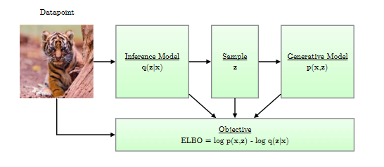
Figure 1: An architecture for a Variational Auto Encoder. (Image source: VAE tutorial, Kingma et.al; 2019)
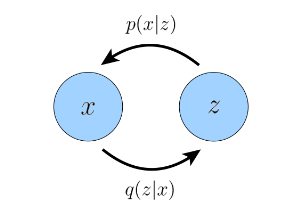
Figure 2: Graphical representation of a Variational Auto Encoder. The $p$ function is the decoder and the $q$ function is the encoder. (Image source: Calvin Luo; 2022)
Figures 1 & 2 give a simplistic representation of a VAE model.
Denoising Diffusion Models
Analogous to VAEs, Denoising Diffusion models also consist of two processes: Diffusion, which is analogous to the VAE encoder, and Denoising, which is analogous to the VAE decoder.
- Diffusion: The diffusion process repeatedly samples random noise and corrupts our input data by adding the noise in $T$ steps. In contrast to the VAE encoder, we typically do not learn this process. At the end of diffusion, at step $T$, the data would be so corrupted that it’s just noise $N(0, I)$.

Figure 3: Illustration of the Diffusion Process. Image of ‘Z’ char is corrupted step by step.
- Denoising: The denoising is done by a learned model that takes completely noisy data and tries to generate the input data by repeatedly (over $t$ steps: $1$ to $T$) removing noise from the noisy data.

Figure 4: Illustration of the Denoising Process. Image of ‘Z’ character is generated step by step.
These models are able to generate images from pure noise.
Humans paint, they are able to generate images in a stepwise manner by painting on a blank canvas. Diffusion models are similar, they generate images in a stepwise manner by denoising a noisy canvas.
At this point, it may be helpful to look at the different models for generative modelling.
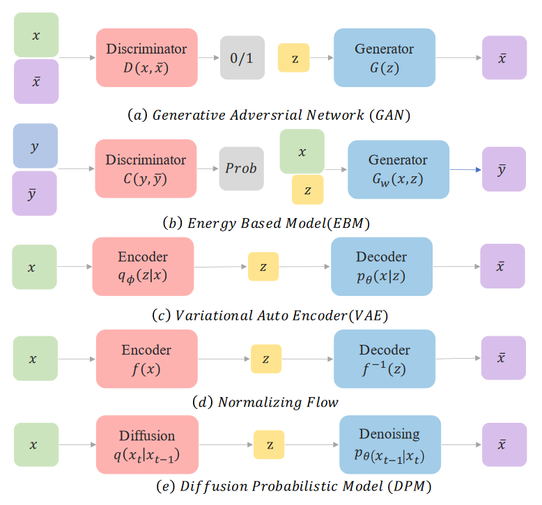
Comparing different generative models. (Image source: Diffusion Models tutorial, Cao et.al; 2022)
Introduction to this series
I have spent too much time understanding diffusion models, which started with some wild posts I saw on Twitter.
Introducing Imagen, a new text-to-image synthesis model that can generate high-fidelity, photorealistic images from a deep level of language understanding. Learn more and and check out some examples of #imagen at https://t.co/RhD6siY6BY pic.twitter.com/C8javVu3iW
— Google AI (@GoogleAI) May 24, 2022
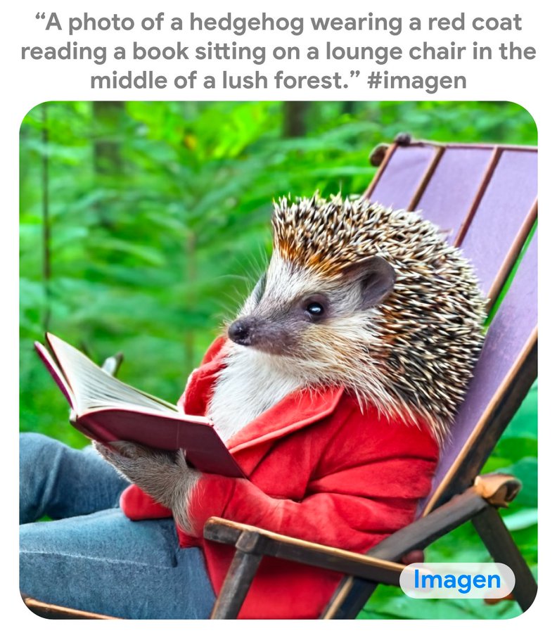
Imagen Google AI Diffusion model. (Image source: Imagen Web Link)
My curiosity led to experiments, which enriched my ML skill-set. In this series, I will try to demystify some magic behind diffusion models.
Finally read a tutorial on Diffusion models. Now, I understand how they work just not why they work. To me it's crazy that they do. pic.twitter.com/LXm5OrD993
— Varun Tulsian (@varuntul22) October 5, 2022
Diffusion Models Series
In this series, I will attempt to simplify diffusion model concepts and provide you with some code that you can easily run on Google Colab or your local Jupyter server. The code requires minimal setup. We will be working on a 2D dataset (generated using scikit-learn) and also the EMNIST dataset (28x28x1 images).
This is the first of 3 posts on diffusion models. You can check all the posts in the Full Diffusion Model Series. All the code for the diffusion model series is available here.
The first 2 parts of the series will focus on setting up the basic concepts and code. You won’t need a GPU to run the code. The code is written in PyTorch.
Part 1: I will introduce the basics of the denoising approach for the diffusion model. We will predict the original distribution directly, following the first part of Luo, 2022.3
Part 2: I will introduce optimizations, predicting error distribution, time step embedding Aka Attention is all you need4, that have been shown to work better. We will also look at class conditioned guidance (classifier free guidance) and steps to generate distributions faster using striding. This will correspond to the second part (Three Equivalent Interpretations) of Luo, 2022.3
- Part 3: In the last part of the series, we will be using the concepts learned to implement diffusion models for character generation by training a U-Net model over the Extended-MNIST dataset. The code is written in JAX, Haiku. This may serve as a good introduction to Jax and Haiku for the uninitiated.
In addition, I have also curated a list of high-quality blogs that I have found helpful, they can be found here.
What are Diffusion Models?
Let’s go over this again, this time in a little more detail. We will start seeing mathematical equations and PyTorch code below.
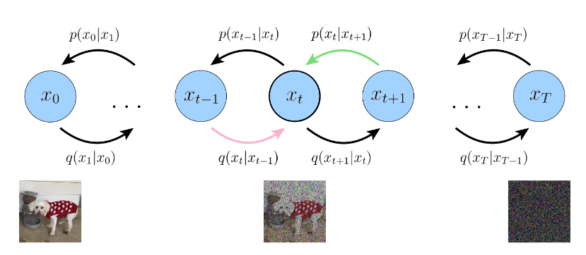
Figure 5: Graphical representation of a Denoising Diffusion Model. The decoder is the $p$ function, the encoder is the $q$ function. (Image source: Calvin Luo; 2022)
Denoising Diffusion models are a Markovian Hierarchical Variational Auto Encoder, unlike a standard VAE model the encoder process (diffusion) and the decoder process (denoising) occur in multiple steps. Figure 5 depicts the diffusion process ($q$), which begins with a random variable $x$ and generates random variables $x_t$ at the $t^{th}$ step. The denoising process ($p$) starts at $x_T$ and attempts to generate $\hat x_t$ and ultimately $\hat x_0$. Let’s call a step in the Diffusion Process as a Diffusion Step, and a step in the Denoising Process as a Denoising Step.
We will be going over the Diffusion Step and the Denoising Step, and the training procedure. But first, let’s build an understanding of what needs to be done to implement such a model.
Training a Denoising Diffusion model
This is the main source of confusion when it comes to understanding diffusion models. From the description above and the analogy with the VAEs, it would seem that training a diffusion model would consist of the following steps.
- Using some data as an input ($x_0$) from the training data.
- Perform a Forward Pass (Diffusion), generating $x_t$’s in $T$ steps.
- Run the noisy image ($x_T$) to the Backward pass (Denoising) to get $\hat x_0$ in $T$ steps. At each step using a $NN(\hat x_t, t)$ and the output should be $\hat x_{t-1}$.
- At the end of the full passes, performing a weight update of the model $NN$ after computing a loss-based $L(x_0, \hat x_0)$.
- Repeat steps 1 through 4.
This would be a perfectly valid approach, however, we can do much better 🙈. First, let’s investigate the issues with this approach. For every input in our dataset, this approach requires us to go through all the time steps, apply diffusion, and then go through the whole denoising steps. The learning (weight updates) only happen at the end of the both the passes. Training in such a way would be slow, and we would not be able to meaningfully learn anything useful.
Instead, we can show that we can effectively learn the distribution $p(X)$ while just doing the following steps.
- Using some data as an input ($x_0$) from the training data.
- Take uniform and random samples of a time variable $t$ ranging from $1,to,T$.
- Compute the latent variable $x_t$ in a single step. Refer to the diffusion step section.
- Apply the $NN$ model to the noisy image ($x_t$) to obtain $\hat x_t^0$. The result of $NN(\hat x_t, t)$ is $\hat x_t^0$. We will not go over each time step. Refer to the denoising step section.
Note about notation: $\hat x_t^0$ is the predicted reconstruction of the input $x_0$ at time step $t$.
- Performing a weight update of the model $NN$ after computing a loss $L(x, \hat x_t^0, t)$.
- Repeat steps 1 through 4.
The proof requires us to reduce the ELBO loss, making use of the Markovian assumption in the diffusion model architecture, and using Monte-Carlo estimates to obtain an equivalent loss. I won’t go into details on this proof, please refer Section: Variational Diffusion Models, equation 100 gives the reduced loss 3. Would highly recommend you do.
We have made significant progress, now we don’t need to go over the entire forward and backward pass before making an update to the model. This will help speed up training significantly.
When we want to generate a new data from noise, we would still go through the full denoising process as it’s helps with the quality of the samples. Generation of new samples through diffusion models is slow. This is an active area of research and various approaches have been proposed to this faster. In my code, I employ time step striding, where we take multiple steps at the same time.
Pseudocode:
| |
1. Diffusion Step
The Diffusion steps add noise to the input vector.
At each time step $t$ in the diffusion process, we sample from the latent variable $x_t$.
One way to do this is the following :
$$
q_t(x_t|x_{t-1}) = N(\sqrt\alpha_tx_{t-1}, (1 - \alpha_t )I)
$$
Note: The diffusion process is annotated as $q$.
At each time step, we are only using $\sqrt\alpha$ times the previous signal $x_{t-1}$ and adds additional noise to the data in a way such that the latent variables stay at a similar scale. We have some additional conditions:
- $\alpha_t$, $t\in[1, T]$, where $\alpha_t < 1$, the diffusion schedule.
- $\alpha_{t-1} < \alpha_t$, as we go along in the diffusion process, we are adding more and more noise.
At this point, let me introduce the re-parameterization trick. $$ N(\sqrt\alpha_tx_{t-1}, (1 - \alpha_t )I) = \sqrt\alpha_tx_{t-1} + (1 - \alpha_t)*\epsilon \quad with \,\, \epsilon \sim N(0, I) $$
The re-paremetarization trick simplifies sampling from a Gaussian distribution. If you want to sample from the diffusion step at $t$, you can simply sample from a standard Gaussian distribution $N(0, I)$ and plug in the mean and variance. Consider another interesting result: suppose we want to sample from the latent $x_t$ ($q(x_t|x_0)$) directly given only the input $x_0$ without having to do it in $t$ steps. We can do so using the re-parameterization trick.
$$
\begin{align}
q(x_t|x_0) &= N(\sqrt\alpha_tx_{t-1}, (1 - \alpha_t )I) \cr
&= \sqrt\alpha_t x_{t-1} + \sqrt{(1-\alpha_t)}\ast\epsilon_t \cr
&= \sqrt\alpha_t(\sqrt\alpha_t x_{t-2} + \sqrt{(1-\alpha_{t-1})}\ast\epsilon_{t-1}) + \sqrt(1-\alpha_t)\ast\epsilon_t \cr
&= \sqrt\alpha_t\sqrt\alpha_t x_{t-2} + \sqrt\alpha_t\sqrt{(1-\alpha_{t-1})}\ast\epsilon_{t-1} + \sqrt(1-\alpha_t)\ast\epsilon_t \cr
&= \sqrt\alpha_t\sqrt\alpha_tx_{t-2} + \sqrt{(1-\alpha_t\alpha_{t-1})}\ast\epsilon_{t-1}^\ast \quad where \thinspace \epsilon_{t-1}^\ast\in N(0, I) \cr
&= ... \cr
&= \sqrt{\bar\alpha_t}x_0 + \sqrt{(1 - \bar\alpha_t )}\ast\epsilon_0^\ast ; \space where \space \bar\alpha_t=\Pi_{i=1}^T{\sqrt\alpha_i}, \space \epsilon_0^\ast \in N(0, I) \cr
&= N(\sqrt{\bar\alpha_t}x_0, (1 - \bar\alpha_t)I)\cr
\end{align}
$$
In equation 5, we have utilized sum of two independent Gaussian random variables.
The latent variable $x_t$ follows a Gaussian distribution, its mean is $\sqrt{\bar\alpha_t}x_0$ and variance is $(1 - \bar\alpha_t)$.
The mean is a function of time step $t$ and the input $x_0$, The variance is only a function of the time step.
With this in place, let’s put some code together.
The diffusion schedule: $\alpha$
| |
Diffusion Step: Given input data $x_0$, a time step $t$ and a schedule, the diffusion method should return the latent variable $x_t$.
In Variational Diffusion Models, Kingma et.al, 20225 propose a way to learn the parameters of the schedule and provide additional insights helpful in understanding diffusion models.
2. Denoising Step
Let’s recap, the denoising process ($p$) is responsible to generate synthetic data $\hat x_0$.
- Start with a completely noisy data, $x_T = N(0, I)$
- Perform a Denoising Step:
- Uses a Neural Network to predict $\hat x_T^0$.
- We will use $\hat x_T^0$ to generate the latent $\hat x_{T-1}$.
- Repeat step 2 with input $\hat x_{T-1}$ to get $\hat x_{T-2}$ until t=1
Refer, our mathematical setup in Figure 5. Let’s look at the mathematical form that a denoising step $p(\hat x_t|\hat x_{t+1})$. This is also called the posterior distribution.
Because the diffusion process is well-defined, let’s work out what a backward transition in the diffusion process: $$ \begin{align} q(x_{t-1}|x_{t}) = \frac{q(x_t|x_{t-1})\ast q(x_{t-1}|x_0)}{q(x_t|x_0)}\quad \text{Baye's theorem \&} \, \text{Note: } x_0 = x \cr = ... \cr \varpropto N(x_{t-1};\underbrace{\frac{\sqrt\alpha_t(1-\bar\alpha_{t-1})x_t + \sqrt{\bar\alpha_{t-1}}(1-\alpha_t)x_0}{1-\bar\alpha_t}}_{\mu_q(x_t,x_0)}, \underbrace{\frac{(1-\alpha_t)(1-\bar\alpha_{t-1})}{1-\bar\alpha_t}I}_{\sum_q(t)}) \cr \end{align} $$ For the full derivation please refer Equation #71; Calvin Luo’s tutorial3
It is convenient to assume that the denoising step $p(\hat x_{t-1}|\hat x_t)$ also follows a Gaussian distribution like the forward process $q(x_{t-1}|x_{t})$. Note: we don’t need to necessarily make this assumption. It’s an inductive bias that we are adding to the system and helps with the stability of training the model or help the model to converge faster.
We will assume the following:
- The mean $\mu_{p(x_{t-1}|x_{t})}$ ($\mu_p$ for short) is dependent on the input $x_0$ ($x_0$ is not known in the denoising step), thus the denoising Neural Network is tasked to make a prediction for the $\hat x_t^0$.
- The variance is not dependent on the data. We will assume it’s fixed and is only a function of the time step, $\sum_{p(x_{t-1}|x_t)} = \sum_q(t)$.
This gives us the following equation for the denoising step: $$ \begin{align} p(\hat x_{t-1}| \hat x_t) \varpropto N(\hat x_{t-1};\frac{\sqrt\alpha_t(1-\bar\alpha_{t-1})\hat x_t + \sqrt{\bar\alpha_{t-1}}(1-\alpha_t)\hat x_t^0}{1-\bar\alpha_t}, \frac{(1-\alpha_t)(1-\bar\alpha_{t-1})}{1-\bar\alpha_t}I) \end{align} $$
As show in Improved Denoising Diffusion Probabilistic Models.6 We could alternatively learn the posterior variance. In this case, we will make the neural network output the variance as well as the mean. If the data is d dimensional, the $NN$ will output 2d dimensions. First d dimensions for the mean, the 2nd d dimensions for the variance.
Diffusion: With Fixed Variance:
| |
3. Training Procedure
We have just defined the diffusion method in the pseudocode. Let’s define the loss function and the Neural Network.
Neural Network:
| |
The input to the Neural Network is 3-dimensional. We are working with 2d dataset, so $\hat x_t$’s is a 2d vector. In this blog post, we are going to pass $t$ as the 3rd dimension, we will pass it as a scalar. In the subsequent posts, we will see how to generate an embedding for a time step and concatenate/fuse it with the input. The output of the $NN$ needs to be $\hat x_t^0$ which is a 2d vector. Refer to the denoising step section. The $NN$ architecture doesn’t really matter. In this case, I’ve used a basic Multi Layer Perceptron with GeLU activation units7. We will use a U-net architecture for character generation using the EMNIST dataset. Checkout Part 3.
Loss Function: At time step $t$ the loss is defined as follows $$ Loss(x_0, \hat x_t, t) = 1/2\ast(\frac{\bar\alpha_{t-1}}{1-\bar\alpha_{t-1}} - \frac{\bar\alpha_t}{1-\bar\alpha_t})\ast\mid\mid x_0-\hat x_0^t\mid\mid_2^2 $$ $$ \text{SNR}_t =\frac{\bar\alpha_t}{1-\bar\alpha_t} $$ SNR stands for Signal to Noise. In the case of the diffusion, the schedule must be chosen such that $SNR_t < SNT_{t-1}$.
Loss:
| |
In Variation Diffusion Models5, authors propose using a separate Neural Network to model SNR as a function of $t$. The Neural Network should be monotonically decreasing. In this setting, we do not need to specify the diffusion schedule, it will be learned along with the diffusion model.
Let’s look at some outputs
In this blog post, we will play with some 2d data-points.
Generating data set for training:
With the code fragments in the blog, you should be able to build your very own diffusion model. You can find the Jupyter Notebook here in case you need some help.
Training Data compared to Diffusion generated data:
Let’s look at data I was able to generate using concepts discussed in this blog.
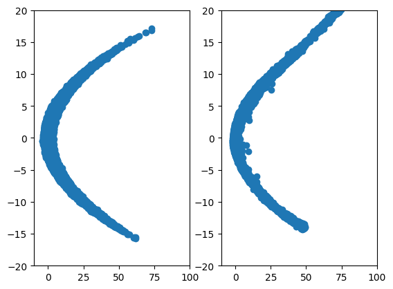
Figure 6: 2D Parabola vs Diffusion generated.
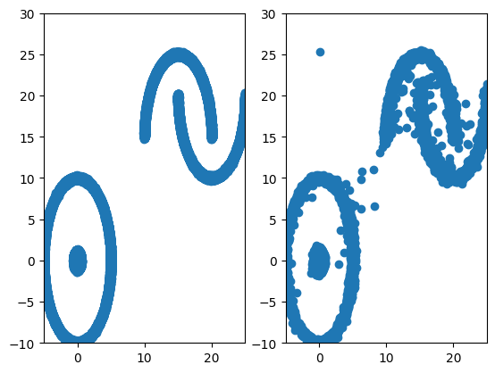
Figure 7: 2D Complex vs Diffusion generated.
Figure 8: A GIF show-casing the denoising process; We start from complete noise and make small improvements step by step.
See you in the next part.
Want to connect? Reach out @varuntul22.
Popov et al. 2021 Grad-TTS: A Diffusion Probabilistic Model for Text-to-Speech ↩︎
Yang et al. 2022 Diffusion Models: A Comprehensive Survey of Methods and Applications ↩︎
Calvin Luo; 2019 “Understanding Diffusion Models: A Unified Perspective” ↩︎ ↩︎ ↩︎ ↩︎
Vaswani et al. 2017 Attention is all you need ↩︎
Kingma et al. 2022 “Variational Diffusion Models” ↩︎ ↩︎
Nichol et al. 2021 Improved Denoising Diffusion Probabilistic Models ↩︎